Navigating the S&P 500 volatility with Hidden Markov Model

Can an HMM model keep us out of turbulent periods?

Recent volatility in the S&P 500 has sparked my curiosity about finding strategies to navigate and potentially avoid such market turbulence. To address this, we will explore the application of a Hidden Markov Model (HMM), a sophisticated statistical tool that could be leveraged to sidestep periods of significant market unrest.

So what is a Hidden Markov Model and why is it applicable in this example? A Hidden Markov Model (HMM) is a statistical model used to represent systems that undergo transitions between hidden states, where the states are not directly observable. Instead, you see observations that are influenced by these hidden states. In our example the observations will be daily returns of the S&P 500 ETF SPY and the two hidden states will be High Volatility and Low Volatility. Low Volatility state will coincide with smaller jumps in prices, while the High Volatility state will mean greater returns but also bigger drawdowns.

There is a saying that stock markets take the ladder up but the elevator down, reflecting the tendency for prices to rise gradually but fall rapidly. Consequently, periods of high volatility are generally those we aim to avoid. High-volatility days tend to cluster together, meaning if today is highly volatile, it is likely that tomorrow will be as well. By identifying a high-volatility day, we can anticipate continued turbulence and opt to stay on the sidelines until the market stabilizes and returns to a lower volatility environment.

As always, full code is provided so that you can experiment with it yourself. Let’s start by getting the data and setting everything up. We also need to install hmmlearn, since it’s not available by default. Our training dataset will last until start of 2019.

import yfinance as yf

df = yf.download('SPY').reset_index()
import pandas as pd
import numpy as np
seed=42
import os
os.environ['PYTHONHASHSEED'] = str(seed)
np.random.seed(seed)
import random
random.seed(seed)
#Tweaking the fonts, etc.
import matplotlib.pyplot as plt
from matplotlib import rcParams

rcParams['figure.figsize'] = (18, 8)
rcParams['axes.spines.top'] = False
rcParams['axes.spines.right'] = False

df.columns = ['_'.join(col).strip() if isinstance(col, tuple) else col
                  for col in df.columns]

df['returns'] = df['Close_SPY'].pct_change().shift(0)
df['pct_change_future'] = df['Close_SPY'].pct_change().shift(-1)

df = df.dropna()
df_train = df[df['Date_'] < '2019-01-01'].reset_index(drop=True)
df_test = df[df['Date_'] >= '2019-01-01'].reset_index(drop=True)
df_train = df_train.dropna()
df_test = df_test.dropna()

Now let’s set up our model and train it on our training dataset.

!pip install hmmlearn

from hmmlearn import hmm
model = hmm.GaussianHMM(n_components=2, covariance_type="diag")
X_train = df_train['returns'].to_numpy().reshape(-1, 1)
model.fit(X_train)

Now that we have a trained model, let’s take a look at what it considers to be high and low volatility periods.

Z_train = model.predict(X_train)
# we want to draw different segments in different colors according to state
fig, ax = plt.subplots(figsize=(10, 5))

# first create arrays with nan
returns0 = np.empty(len(Z_train))
returns1 = np.empty(len(Z_train))
returns0[:] = np.nan
returns1[:] = np.nan

# fill in the values only if the state is the one corresponding to the array
returns0[Z_train == 0] = df_train['returns'][Z_train == 0]
returns1[Z_train == 1] = df_train['returns'][Z_train == 1]
plt.plot(returns0, label='state 0')
plt.plot(returns1, label='state 1')
plt.legend();

The screenshot above clearly shows that the majority of observations are classified as state 0 (low volatility) while bigger returns correspond to state 1 (high volatility) and are much more rare. Notice that our earlier guess that days with high volatility will be clustered around each other also seems to be true. However, there is an issue with the screenshot above. There are several instances where the model ping-pongs between state 1 and state 0, which would make it a hassle in a real trading strategy. Let’s take a look at the model’s transition matrix.

My goal is to provide you with the tools that will give you an edge in the markets. Follow the link below to get 10% off for the next 12 months.

Become a paid subscriber to receive:

• Trading indicators and strategies. Full, ready-to-use code for your investing — no black boxes or holy grails, just full transparency and ownership of your advantage.

• Weekly newsletter covering current market conditions. Analysis on economic trends, key data releases, and actionable insights to stay ahead of market shifts.

# transition matrix
model.transmat_

The transition matrix defines the probabilities of moving between these hidden states. Each element transmat_[i, j] represents the probability of transitioning from state i to state j. For example, when we are in state 0 there is a 92% chance that we will stay in this state. In order to make the model more stable we will modify the transition matrix, so that there is a 99% chance of staying in the same state.

# try to set the transition matrix intuitively
model.transmat_ = np.array([
  [0.999, 0.001],
  [0.001, 0.999],
])

By adjusting the transition matrix, we're influencing how the model believes the market switches between its underlying states. Note that this doesn’t necessarily mean that the model will almost never switch from one state to the other. The model still switches between the hidden states even with the transition matrix set to favor staying in the same state. This is because the transition matrix only influences the probability of switching states, not whether a switch can happen. The model combines the emission probabilities (likelihood of the observed return given each state) and the transition probabilities (likelihood of switching or staying in a state) to determine the most likely sequence of hidden states that generated the observed data. If the model encounters a return that is very unlikely to be generated by the current state (e.g., a large positive return in a "low-volatility" state), it might still switch states, even if the transition probability is low. This is because the emission probability for the other state might be significantly higher. Let’s see how that changes the previous chart.

# run inference again
Z_train = model.predict(X_train)

fig, ax = plt.subplots(figsize=(10, 5))

# first create arrays with nan
returns0 = np.empty(len(Z_train))
returns1 = np.empty(len(Z_train))
returns0[:] = np.nan
returns1[:] = np.nan

# fill in the values only if the state is the one corresponding to the array
returns0[Z_train == 0] = df_train['returns'][Z_train == 0]
returns1[Z_train == 1] = df_train['returns'][Z_train == 1]
plt.plot(returns0, label='state 0')
plt.plot(returns1, label='state 1')
plt.legend();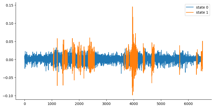

Now we can clearly see that the model doesn’t jump around nearly as often. By setting the transition probabilities to be very high for staying in the same state, we are essentially telling the model to be more "conservative" in its state switching. It will only switch states if there's strong evidence (from the observed returns) that the market has actually changed its underlying behavior.

This results in smoother transitions between states and reduces the "jumping around" that we saw with a more balanced transition matrix, making it much easier to actually implement in trading.

Now let’s see what the model’s output is for the test dataset.

Z_test_iterative = []

equity_hmm_iterative = [1.0] 

# Iterate through the test set day by day
for i in range(len(df_test)):
    X_test_subset = df_test['returns'].iloc[:i+1].to_numpy().reshape(-1, 1)
    current_state = model.predict(X_test_subset)[-1]
    Z_test_iterative.append(current_state)


    signal = 1 if current_state == 0 else 0

    daily_return_hmm = signal * df_test['pct_change_future'].iloc[i]

    
    equity_hmm_iterative.append(equity_hmm_iterative[-1] * (1 + daily_return_hmm))


Z_test_iterative = pd.Series(Z_test_iterative, index=df_test.index)
equity_hmm_iterative = pd.Series(equity_hmm_iterative, index=[df_test.index[0]] + list(df_test.index))

df_test['state_iterative'] = Z_test_iterative
df_test['signal_iterative'] = np.where(df_test['state_iterative'] == 0, 1, 0)
df_test['equity_HMM_iterative'] = equity_hmm_iterative.iloc[1:]
df_test['equity_buy_and_hold'] = np.cumprod(1+df_test['pct_change_future'])

fig, ax = plt.subplots(figsize=(10, 5))

# first create arrays with nan
returns0 = np.empty(len(Z_test_iterative))
returns1 = np.empty(len(Z_test_iterative))
returns0[:] = np.nan
returns1[:] = np.nan

returns0[Z_test_iterative == 0] = df_test['returns'][Z_test_iterative == 0]
returns1[Z_test_iterative == 1] = df_test['returns'][Z_test_iterative == 1]
plt.plot(returns0, label='state 0')
plt.plot(returns1, label='state 1')
plt.legend();

This looks pretty good: the model has three clearly-defined periods that are considered high-volatility.

Now let’s create a trading system based on HMM’s output. In this example we will either stay invested in SPY or close out our long position and wait. If the model considers today to be a high volatility day we close our position and stay out of the market the next day. If today is a low volatility day we do nothing and keep our position open for tomorrow.

from plotly import graph_objects as go
fig = go.Figure()

fig.add_trace(
    go.Line(x=df_test['Date_'], y=df_test['equity_buy_and_hold'], name='Buy and Hold')
)

fig.add_trace(
    go.Line(x=df_test['Date_'], y=df_test['equity_HMM_iterative'], name='HMM')
)

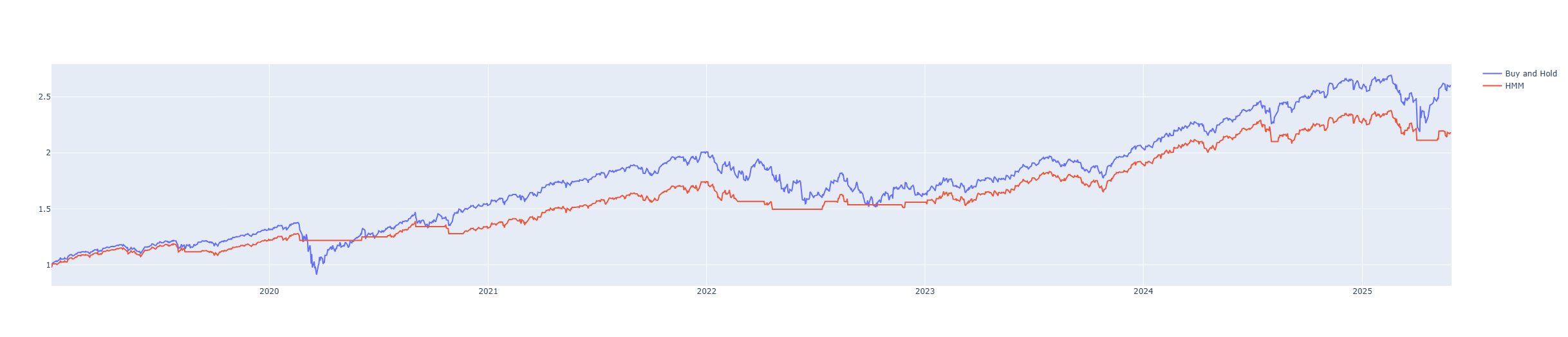
The model did reasonably well: it stayed out for most of the 2020 crash, as well as nearly the entirety of 2022 and the recent tariff selloff. Let’s see what its drawdown and CAGR look like.

def get_max_drawdown(col):
    drawdown = col / col.cummax() - 1
    return '{:.2f}'.format(100 * drawdown.min())

def calculate_cagr(col, n_years):
    cagr = (col.values[-1] / col.values[0]) ** (1 / n_years) - 1
    return '{:.2f}'.format(100 * cagr)

print('Maximum Drawdown Buy and Hold:', get_max_drawdown(df_test['equity_buy_and_hold']))
print('Maximum Drawdown HMM:', get_max_drawdown(df_test['equity_HMM_iterative']))
n_years = (df_test['Date_'].max() - df_test['Date_'].min()).days / 365.25

print('CAGR Buy and Hold:', calculate_cagr(df_test['equity_buy_and_hold'].dropna(), n_years))
print('CAGR HMM:', calculate_cagr(df_test['equity_HMM_iterative'].dropna(), n_years))

While the model ended up with lower CAGR, it managed to cut the max drawdown by more than 2x.

Overall, Hidden Markov Models (HMMs) can be a very valuable tool in trading. For instance, the model discussed in this post can serve as an effective risk management strategy by helping investors avoid turbulent periods in the market.

My goal is to provide you with the tools that will give you an edge in the markets. Follow the link below to get 10% off for the next 12 months.

Become a paid subscriber to receive:

• Trading indicators and strategies. Full, ready-to-use code for your investing — no black boxes or holy grails, just full transparency and ownership of your advantage.

• Weekly newsletter covering current market conditions. Analysis on economic trends, key data releases, and actionable insights to stay ahead of market shifts.

If you find this content useful, consider subscribing. I plan to explore many other strategies and instruments that can help elevate your trading skills. Subscribe and follow along for more insights!

Make sure to check my other posts:

Walk-Forward Validation: A Stress Test for Your Trading Strategy

Can SARSA algorithm improve our trading strategy?