The Golden Age of Forecasting: Machine Learning and Gold Price Prediction

Gold has been on a tear this year. Could we "mine" even more value out of it?

In this post we continue to explore the use of machine learning to predict the performance of financial assets and level up our approach to investing. This time we are taking a detour away from stocks to take a look at an entirely different asset: gold futures. Gold’s performance has been very strong recently and beating the buy-and-hold approach would be quite challenging, making it a good test. In this post I will be comparing the performance of multiple models, including some that I haven’t tried yet in my other posts, such as CatBoost and LightGBM. As usual, I will be providing the full code so that you could try it out yourself. Every new post builds on my previous posts, so if you want to see some more commentary regarding some part of the code, I encourage you to check out my previous posts.

The code below pulls the prices of gold futures from Yahoo Finance and adds the necessary features that would be used in the models.

import yfinance as yf

df = yf.download('GC=F').reset_index()
import pandas as pd
import numpy as np
seed=42
import os
os.environ['PYTHONHASHSEED'] = str(seed)
np.random.seed(seed)
import random
random.seed(seed)
#Tweaking the fonts, etc.
import matplotlib.pyplot as plt
from matplotlib import rcParams

rcParams['figure.figsize'] = (18, 8)
rcParams['axes.spines.top'] = False
rcParams['axes.spines.right'] = False
# Feature deriving

# Distance from the moving averages
for m in [10, 20, 30, 50, 100]:
    df[f'feat_dist_from_ma_{m}'] = df['Close']/df['Close'].rolling(m).mean()-1

# Distance from n day max/min
for m in [3, 5, 10, 15, 20, 30, 50, 100]:
    df[f'feat_dist_from_max_{m}'] = df['Close']/df['High'].rolling(m).max()-1
    df[f'feat_dist_from_min_{m}'] = df['Close']/df['Low'].rolling(m).min()-1

# Price distance
for m in [1, 2, 3, 4, 5, 10, 15, 20, 30, 50, 100]:
    df[f'feat_price_dist_{m}'] = df['Close']/df['Close'].shift(m)-1



# Relative Strength Index (RSI) - 14 days
def calculate_rsi(series, window=14):
    series_copy = series.copy()  # Work with a copy
    diff = series_copy.diff(1)
    gain = np.where(diff > 0, diff, 0)
    loss = np.where(diff < 0, -diff, 0)

    avg_gain = pd.Series(gain).rolling(window=window, min_periods=14).mean()
    avg_loss = pd.Series(loss).rolling(window=window, min_periods=14).mean()

    rs = avg_gain / avg_loss
    rsi = 100 - (100 / (1 + rs))

    df.loc[:, 'feat_rsi_14'] = rsi  # Use .loc to explicitly modify the DataFrame

# Call the function with the 'Close' column
calculate_rsi(df['Close'])

# Price change over the last 5 and 10 days
df['feat_price_change_5'] = df['Close'].pct_change(periods=5)
df['feat_price_change_10'] = df['Close'].pct_change(periods=10)

# 1 day performance
df['pct_change_future'] = df['Close'].pct_change().shift(-1)
# Calculate cumulative growth of $100 investment
df['Change_100_Investment'] = (1 + df['pct_change_future']).cumprod() * 100
# Adding a new column 'target' based on pct_change_future
df['target'] = np.where(df['pct_change_future'] > 0, 1, 0)

Now we clean up the data and split it into training, validation and test sets. After that we scale the data on the training set and apply the scaling to the validation and test sets.

df = df.dropna()

# Define the date ranges for training, validation, and testing
validation_start_date = '2015-01-01'
validation_end_date = '2019-01-01'

# Split the DataFrame into training, validation, and testing sets
df_train = df[df['Date'] < validation_start_date].reset_index(drop=True)
df_val = df[(df['Date'] >= validation_start_date) & (df['Date'] < validation_end_date)].reset_index(drop=True)
df_test = df[df['Date'] >= validation_end_date].reset_index(drop=True)

feat_cols = [col for col in df.columns if 'feat' in col]

df_train = df_train.dropna()
df_val = df_val.dropna()
df_test = df_test.dropna()

from sklearn.preprocessing import StandardScaler
scaler = StandardScaler()
x_train = df_train[feat_cols]
x_train_scaled = scaler.fit_transform(x_train)
x_train_scaled_df = pd.DataFrame(x_train_scaled, columns=feat_cols)
x_test = df_test[feat_cols]
x_test_scaled = scaler.transform(x_test)
x_test_scaled_df = pd.DataFrame(x_test_scaled, columns=feat_cols)
x_val = df_val[feat_cols]
x_val_scaled = scaler.transform(x_val)
x_val_scaled_df = pd.DataFrame(x_val_scaled, columns=feat_cols)

x_train = x_train_scaled_df
x_test = x_test_scaled_df
x_val = x_val_scaled_df
y_train = df_train['target']
y_test = df_test['target']
y_val = df_val['target']

Now, we install the necessary packages for CatBoost as well as importing the libraries for the models we will use. We also introduce code for hyperparameter tuning with GridSearchCV. The point of this is to try out different combinations of parameters introduced in the param_grid below and find the combination with best accuracy. We then use the best set of parameters to fit the model and finally make predictions on the test set. We first do it for the XGBoost model.

My goal is to provide you with the tools that will give you an edge in the markets. Follow the link below to get 10% off for the next 12 months.

Become a paid subscriber to receive:

• Trading indicators and strategies. Full, ready-to-use code for your investing — no black boxes or holy grails, just full transparency and ownership of your advantage.

• Weekly newsletter covering current market conditions. Analysis on economic trends, key data releases, and actionable insights to stay ahead of market shifts.

!pip install catboost
# Import necessary libraries
from sklearn.model_selection import GridSearchCV
from sklearn.metrics import accuracy_score
from xgboost import XGBClassifier
from sklearn.ensemble import RandomForestClassifier
from catboost import CatBoostClassifier
from lightgbm import LGBMClassifier
from sklearn.metrics import accuracy_score


# Hyperparameter tuning for XGBoost
param_grid_xgb = {
    'max_depth': [3, 5, 7],
    'learning_rate': [0.1, 0.01, 0.001],
    'n_estimators': [50, 75, 100],
}

xgb_model = XGBClassifier()

grid_search_xgb = GridSearchCV(estimator=xgb_model, param_grid=param_grid_xgb, cv=3, scoring='accuracy', n_jobs=-1)
grid_search_xgb.fit(x_train, y_train)

# Best parameters for XGBoost
best_params_xgb = grid_search_xgb.best_params_

# Train XGBoost model with best parameters
xgb_model_best = XGBClassifier(**best_params_xgb)
xgb_model_best.fit(x_train, y_train, eval_set=[(x_val, y_val)], eval_metric='error', early_stopping_rounds=50, verbose=True)

print("Best Parameters for XGBoost:", best_params_xgb)
# Predictions on test set
y_pred_xgb = xgb_model_best.predict(x_test)
accuracy_xgb = accuracy_score(y_test, y_pred_xgb)
print("XGBoost Test Accuracy:", accuracy_xgb)

Now we do the same procedure for the Random Forest, CatBoost and LightGBM models. CatBoost is a gradient boosting algorithm developed by Yandex, it has shown good performance in various tasks, including classification, which is why it’s interesting to see its performance here. LightGBM (Light Gradient Boosting Machine) is another gradient boosting framework (this one is developed by Microsoft).

# Hyperparameter tuning for RandomForest
param_grid_rf = {
    'n_estimators': [50, 75, 100],
    'max_depth': [3, 5, 7],
}

rf_model = RandomForestClassifier()

grid_search_rf = GridSearchCV(estimator=rf_model, param_grid=param_grid_rf, cv=3, scoring='accuracy', n_jobs=-1)
grid_search_rf.fit(x_train, y_train)

# Best parameters for RandomForest
best_params_rf = grid_search_rf.best_params_

# Train RandomForest model with best parameters
rf_model_best = RandomForestClassifier(**best_params_rf)
rf_model_best.fit(x_train, y_train)

# Predictions on test set
y_pred_rf = rf_model_best.predict(x_test)
accuracy_rf = accuracy_score(y_test, y_pred_rf)
print("Random Forest Test Accuracy:", accuracy_rf)

# Hyperparameter tuning for CatBoost
param_grid_catboost = {
    'depth': [3, 5, 7],
    'learning_rate': [0.1, 0.01, 0.001],
    'iterations': [50, 75, 100],
}

catboost_model = CatBoostClassifier(silent=True)

grid_search_catboost = GridSearchCV(estimator=catboost_model, param_grid=param_grid_catboost, cv=3, scoring='accuracy', n_jobs=-1)
grid_search_catboost.fit(x_train, y_train, verbose=False)

# Best parameters for CatBoost
best_params_catboost = grid_search_catboost.best_params_

# Train CatBoost model with best parameters
catboost_model_best = CatBoostClassifier(**best_params_catboost, silent=True)
catboost_model_best.fit(x_train, y_train, eval_set=(x_val, y_val), use_best_model=True, verbose=True)

# Predictions on test set
y_pred_catboost = catboost_model_best.predict(x_test)
accuracy_catboost = accuracy_score(y_test, y_pred_catboost)
print("CatBoost Test Accuracy:", accuracy_catboost)

# Hyperparameter tuning for LightGBM
param_grid_lgb = {
    'max_depth': [3, 5, 7],
    'learning_rate': [0.1, 0.01, 0.001],
    'n_estimators': [50, 75, 100],
}

lgb_model = LGBMClassifier()

grid_search_lgb = GridSearchCV(estimator=lgb_model, param_grid=param_grid_lgb, cv=3, scoring='accuracy', n_jobs=-1)
grid_search_lgb.fit(x_train, y_train)

# Best parameters for LightGBM
best_params_lgb = grid_search_lgb.best_params_

# Train LightGBM model with best parameters
lgb_model_best = LGBMClassifier(**best_params_lgb)
lgb_model_best.fit(x_train, y_train, eval_set=(x_val, y_val))

# Predictions on test set
y_pred_lgb = lgb_model_best.predict(x_test)
accuracy_lgb = accuracy_score(y_test, y_pred_lgb)
print("LightGBM Test Accuracy:", accuracy_lgb)

Finally, we use the models to make predictions on our test set, and graph the results for each model.

y_test_xgb = (y_pred_xgb > 0.5).astype(int)
df_test['xgb_pred'] = y_test_xgb
y_test_rf = (y_pred_rf > 0.5).astype(int)
df_test['rf_pred'] = y_test_rf
y_test_cat = (y_pred_catboost > 0.5).astype(int)
df_test['cat_pred'] = y_test_cat
y_test_light = (y_pred_lgb > 0.5).astype(int)
df_test['light_pred'] = y_test_light

df_test['equity_xgb'] = np.cumprod(1+df_test['xgb_pred']*df_test['pct_change_future'])
df_test['equity_rf'] = np.cumprod(1+df_test['rf_pred']*df_test['pct_change_future'])
df_test['equity_cat'] = np.cumprod(1+df_test['cat_pred']*df_test['pct_change_future'])
df_test['equity_light'] = np.cumprod(1+df_test['light_pred']*df_test['pct_change_future'])
df_test['equity_buy_and_hold'] = np.cumprod(1+df_test['pct_change_future'])

from plotly import graph_objects as go
fig = go.Figure()

fig.add_trace(
    go.Line(x=df_test['Date'], y=df_test['equity_buy_and_hold'], name='Buy and Hold')
)

fig.add_trace(
    go.Line(x=df_test['Date'], y=df_test['equity_xgb'], name='XGB')
)

fig.add_trace(
    go.Line(x=df_test['Date'], y=df_test['equity_rf'], name='Random Forest')
)
fig.add_trace(
    go.Line(x=df_test['Date'], y=df_test['equity_cat'], name='CAT')
)
fig.add_trace(
    go.Line(x=df_test['Date'], y=df_test['equity_light'], name='Light')
)
fig.update_layout(
    title_text='Models Backtest',
    legend={'x': 0, 'y':-0.05, 'orientation': 'h'},
    xaxis={'title': 'Date'},
    yaxis={'title': 'Multiple from Initial Investment'}
)

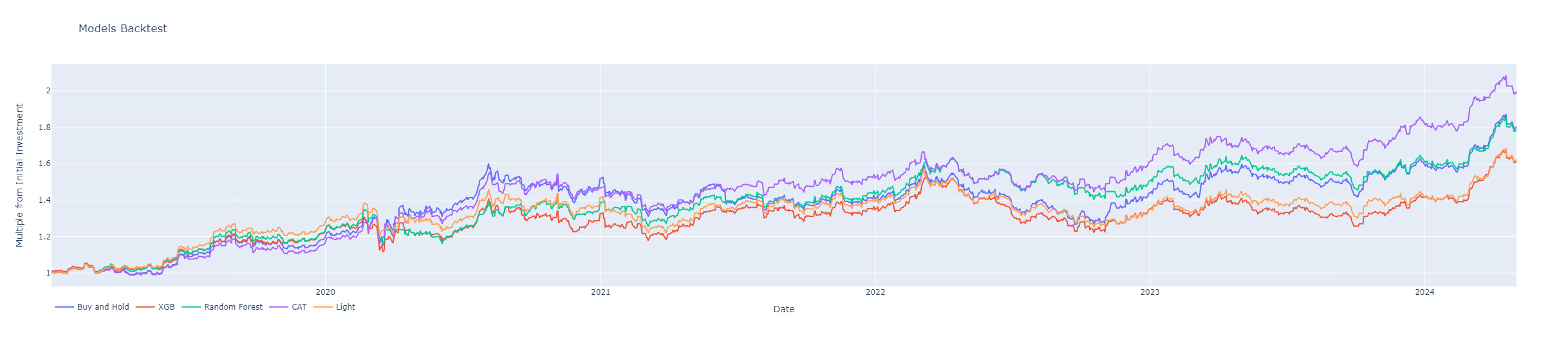
At first glance it seems pretty clear that the CatBoost model is the winner here, beating all the other models and also gold itself in terms of pure returns. Let’s also take a look at each of the model’s CAGR and drawdowns.

def get_max_drawdown(col):
    drawdown = col / col.cummax() - 1
    return '{:.2f}'.format(100 * drawdown.min())

def calculate_cagr(col, n_years):
    cagr = (col.values[-1] / col.values[0]) ** (1 / n_years) - 1
    return '{:.2f}'.format(100 * cagr)

print('Maximum Drawdown Buy and Hold:', get_max_drawdown(df_test['equity_buy_and_hold']))
print('Maximum Drawdown XGBoost:', get_max_drawdown(df_test['equity_xgb']))
print('Maximum Drawdown Random Forest:', get_max_drawdown(df_test['equity_rf']))
print('Maximum Drawdown CATBoost:', get_max_drawdown(df_test['equity_cat']))
print('Maximum Drawdown LightGBM:', get_max_drawdown(df_test['equity_light']))
print('')

n_years = (df_test['Date'].max() - df_test['Date'].min()).days / 365.25

print('CAGR Buy and Hold:', calculate_cagr(df_test['equity_buy_and_hold'].dropna(), n_years))
print('CAGR XGBoost:', calculate_cagr(df_test['equity_xgb'].dropna(), n_years))
print('CAGR Random Forest:', calculate_cagr(df_test['equity_rf'].dropna(), n_years))
print('CAGR CATBoost:', calculate_cagr(df_test['equity_cat'].dropna(), n_years))
print('CAGR LightGBM:', calculate_cagr(df_test['equity_light'].dropna(), n_years))

Again, CatBoost is the best performer all-around, with highest CAGR and lowest drawdown. It’s pretty encouraging to see this performance: gold has been in a pretty clear uptrend over the entire test data set with only one prolonged drawdown episode, so beating the buy-and-hold performance in this case is a pretty big win. I encourage readers to experiment with the code, try it out and see what insights it could bring.

These posts are meant to be an introduction into the world of trading and investing using the full array of tools available to any retail investor and will slowly increase in complexity, so make sure to subscribe and follow along!

My goal is to provide you with the tools that will give you an edge in the markets. Follow the link below to get 10% off for the next 12 months.

Become a paid subscriber to receive:

• Trading indicators and strategies. Full, ready-to-use code for your investing — no black boxes or holy grails, just full transparency and ownership of your advantage.

• Weekly newsletter covering current market conditions. Analysis on economic trends, key data releases, and actionable insights to stay ahead of market shifts.